I need a plan

Here’s the plan. I want to create a movie which shows some nearby points spread out over the full space of a Lorenz attractor. I’d like to make a proper movie with sharp graphics and fluid motion. I want to write all my code in R, and I’d like it to render in five or ten minutes on my 4 core i5 laptop.

So the plan is to make a 1080p (1920x1080) movie at 25 frames per second, each frame rendered with {ggplot2}.

Still loving you

First, I need to create each still image. Let’s make a function to generate the path of a single particle through the Lorenz system.

library(tidyverse)
library(deSolve)

generate_lorenz <- function(
  start_coords = c(x = 1, y = 1, z = 1),
  iterations = 100
) {
  deSolve::ode(
    y = start_coords,
    times = seq(0, iterations / 100, length.out = iterations),
    parms = list(
      rho = 28,
      sigma = 10,
      beta = 8/3
    ),
    func = function(time, state, params) {
      with(as.list(c(state, params)), {
        dx = sigma * (y - x)
        dy = x * (rho - z) - y
        dz = x * y - beta * z
        
        list(c(dx, dy, dz))
      })
    }
  ) %>%
    as.data.frame() %>%
    mutate(iteration = row_number()) %>%
    select(-time)
}

I won’t go over the gritty details of {deSolve} – in short it generates the path defined by a differential equation. I could have chosen the simpler Euler integration to do this. On the other hand, the different pieces of the differential equation is clearer this way, once you get your head around what it does. If you look up the algorithm for the Lorenz attractor, I’m sure you’ll recognize the important bits.

generate_lorenz() will generate the path of a single point. Since I want to track a bunch of them, I need to run it for each point:

points <- tibble(id = 1:250) %>%
  mutate(trace = map(id, function(id) {
    generate_lorenz(
      start_coords = c(x = 1 + rnorm(1, 0, 0.5), y = 3 + rnorm(1, 0, 0.5), z = 21  + rnorm(1, 0, 0.5)),
      iterations = 90*25)
  })) %>%
  unnest(trace)

head(points)

## # A tibble: 6 x 5
##      id     x     y     z iteration
##   <int> <dbl> <dbl> <dbl>     <int>
## 1     1 0.821  2.16  21.5         1
## 2     1 0.951  2.20  20.9         2
## 3     1 1.07   2.25  20.4         3
## 4     1 1.19   2.32  19.9         4
## 5     1 1.30   2.40  19.4         5
## 6     1 1.41   2.49  18.9         6

There’s already a bunch of decisions embedded in the code above:

• The step size is 1/100 of a unit in generate_lorenz()
• I add 250 points
• … that start at roughly c(x = 1, y = 3, z = 21)
• … normally distributed round this point
• I run the animation for 90 seconds at 25 frames per second

As you might expect, I didn’t set these parameters on the first attempt, but went back and forth with different settings until I was happy with the results. For example, after having run the animation a couple of times I chose a low-speed starting point to have a not too-jerky start to the animation. Playing around is my way of figuring this out.

Whole plotta love

With 562500 point at my disposal, time to get some digital ink on disk. I write a function to plot a single frame. This turned out to be super useful when calibrating the parameters above: with this function I would for example plot frame 250 to see how the animation would look 250/25 = 10 seconds in.

I plot the Lorenz attractor only in the (x, y) plan. Adding some rotation to it would make the movie more interesting. For the purpose of learning the technical details of making an animation this is enough.

plot_tick <- function(points, tick) {
  xrange <- range(points$x)
  yrange <- range(points$y)
  
  points %>%
    filter(iteration >= tick - 30, iteration <= tick) %>%
    group_by(id) %>%
    mutate(xend = lag(x),
           yend = lag(y)) %>%
    filter(!is.na(xend),
           !is.na(yend)) %>%
    ggplot(aes(x, y, color = sqrt(abs(iteration - tick)))) +
      geom_segment(aes(xend = xend, yend = yend, alpha = iteration - tick)) +
      geom_point(data = filter(points, iteration == tick), aes(alpha = 0), size = 0.25) +
      scale_x_continuous(limits = xrange) +
      scale_y_continuous(limits = yrange) +
      scale_alpha_continuous(range = c(0.1, 0.7)) +
      scale_color_gradientn(colors = c("#E8DDCB", "#CDB380", "#036564", "#033649", "#031634")) +
      theme_void() +
      theme(
        plot.background = element_rect(fill = 'black'),
        legend.position = 'none'
      )
}

plot_tick(points, 225)

I leave a 30 iteration trail behind each point as a geom_segment(). The alpha fades out to more transparent and the color fades out to darker towards the tail. I add a small geom_point() to each point’s head. I set the x and y limits of the axis to the whole range of visited points, to make sure the coordinates stay in the same place throughout the animation. As for alpha levels and color schemes, you guessed it: tinkering. The palette is from Colourlovers – an amazing page to find cool palettes, which also has a {colourlovers} package to work with in R.

Let’s work together

Now, time go generate a bunch of frames! I’m looking to plot 90 * 25 = 2250 of these, and I don’t want to do it one at a time. There’s a bunch of packages to do parallel computing in R. I prefer to use {future} and {furrr} with tidy data, but sometimes they just don’t seem to play nicely with me (probably my fault). Today, I’ll go with parallel::mclapply(), in a nice wrapper that gives a progress bar.

library(parallel)
library(pbmcapply)
options(mc.cores = parallel::detectCores())

# if (FALSE) to make this blog post render.
# Run the inner part!
if (FALSE) {
  foo <- pbmclapply(unique(points$iteration), function(tick) {
    p <- plot_tick(points, tick)
      
    ggsave(sprintf('~/tmp/anim/%04d.png', tick), plot = p, width = 2*19.2/2, height = 2*10.8/2, dpi=200, antialias = "subpixel")
  })
}

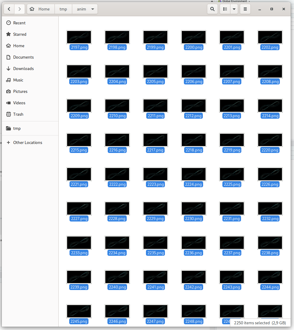
In short: kick off one process on each core and have each render a frame at a time. I save each plot to a directory I created (~/tmp/anim) as a 3840x2160 png image. (Yes, again tinkering to get the settings right).

Some six minutes later, I’ve got 2250 files adding up to just short of 3 GB waiting for me.

Stiching it up

Finally, I stitch the images together into a 90 second clip using ffmpeg. Here’s where I spent a ton of time on Google trying to get the final video to look sharp. A few important settings I came across:

• -vf “fade=t=out:st=88:d=2” - fade out the image starting at second 88 for two seconds.
• -vf “scale=1920:-1” - make the resolution 1920x(whatever keeps the aspect ratio): for us meaning a 1080p resolution.
• -crf 0 - A low number means little compression = larger files but sharper images. In the end, this is what I think got the trick done.

$ cd ~/tmp/anim
$ ffmpeg -i %04d.png -vf "fade=t=out:st=88:d=2,scale=1920:-1" -c:v libx264 -preset slow -crf 0 -pix_fmt yuv420p output.mkv

Another three or four minutes later, I have a video waiting for me – a good 360 MB in size.

You can view the final result on Youtube. Don’t forget to pick HD 1080p quality now that my poor computer struggled so hard for it!

Lessons learned

• It was a lot trickier to get sharp-ish video than I expected. I’m sure reading some manual could have saved me some time.
• Writing a function to render a single frame made it really convenient to debug / find the right parameters for the animation.
• Running parallelizable things in parallel on many cores makes things fast!
• I still haven’t found a good way to animate things in R.