Here’s another neat trick I picked up from Julien Sprott’s book on Strange Attractors: that good ole’ 90s 3D effect you get if you focus outside of the image and frustratingly wait for that image to appear.
The technique I will use is called Cross-eyed stereo viewing, which works by the viewer crossing their eyes inwards. Let’s start with an example to see where we’re going.
To generate pretty pictures, I will mostly use the same technique as in my post about 2D quadratic iteraded map attractors, but now for 3D dittos. In short: I will use the quadratic_3d() function to generate interesting 3D data to plot.
library(tidyverse)
theme_set(theme_void() + theme(legend.position = 'none'))

quadratic_3d <- function(a, x, y, z) {
  xn1 <- a[ 1] + a[ 2]*x + a[ 3]*x*x + a[ 4]*x*y + a[ 5]*x*z + a[ 6]*y + a[ 7]*y*y + a[ 8]*y*z + a[ 9]*z + a[10]*z*z
  yn1 <- a[11] + a[12]*x + a[13]*x*x + a[14]*x*y + a[15]*x*z + a[16]*y + a[17]*y*y + a[18]*y*z + a[19]*z + a[20]*z*z
  zn1 <- a[21] + a[22]*x + a[23]*x*x + a[24]*x*y + a[25]*x*z + a[26]*y + a[27]*y*y + a[28]*y*z + a[29]*z + a[30]*z*z

  c(xn1, yn1, zn1)
}

iterate <- function(step_fn, a, x0, y0, z0, iterations) {
  x <- rep(x0, iterations)
  y <- rep(y0, iterations)
  z <- rep(z0, iterations)

  for(n in 1:(iterations - 1)) {
    xyz <- step_fn(a, x[n], y[n], z[n])
    x[n+1] <- xyz[1]
    y[n+1] <- xyz[2]
    z[n+1] <- xyz[3]
  }

  tibble(x = x, y = y, z = z) %>%
    mutate(n = row_number())
}

normalize_xyz <- function(df) {
  range <- with(df, max(max(x) - min(x), max(y) - min(y), max(x) - min(z)))

  df %>%
    mutate(x = (x - min(x)) / range,
           y = (y - min(y)) / range,
           z = (z - min(z)) / range)

}
I will show you how to use the code above in a bit. First though, let’s practice on a picture!
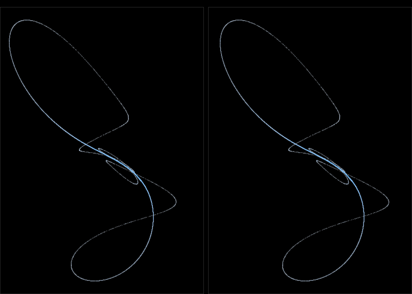
This is a stereo image. Even though the two copies look very much alike, there are subtle differences between them. When you look at them the right way, a third image will appear that magically combinees them into a single 3D image. Here’s how I do to see it.
I slightly cross my eyes while watching emptily in the distance “through” the image. As I do, I start to see doubles making for four strings in total. Now I need to put two of these on top of each others which takes some frustrating practice. Here’s a few tips.
- Look for a sharp edge or distinct path that you aim to match up.
- To see which two strings you are supposed to put on top of each others, try to rotate the screen as a steering wheel. This makes the target strings shift vertically (up and down).
- I first try to get the strings roughly aligned horizontally. If I can’t manage that, the image might be too large for my eyes to cross enough. A horizontal (X-axis) distance between matching points on the two strings should be somewhere around 4-6 cm. For the image above, a total image width of 8-9 cm seems good to me with my screen in my lap, some 60 cm from my eyes. If the size is wrong you can resize your browser, or try a mobile screen, or…
- When the horizontal axis align, I focus on my edge and turn my screen steering-wheel-style to match my edge up. When I get close enough, my eyes magically lock in on the joint 3D picture!
- If you’ve just spent lots of time reading, your eyes are set on a whole other focus. Close your eyes for half a minute or so to help them reset.
Hopefully you’ll get it; if not you might want to try Google. It took me some time to get it first, but it gets much easier with practice and during a session!
That sweet stereo
The technique to render these images is surprisingly easy. The basis of you being able to see in three dimensions at all is that your eyes are placed slightly appart. When you look at a scene, the 2D projection that enters one eye is slightly different from the one to the other eye. When we here shift our two images in the right way, we “pre-process” the 3D-to-2D image entering each eye, which creates the illusion of depth.

As a walk-through example, I’ll use another plot: the Lorenz Attractor. First we need to generate the (x, y, z) points
lorenz <- function(iterations, sigma = 10, rho = 28, beta = 8/3, x0 = 0.5, y0 = 1, z0 = 1.2, dt = 0.01) {
  x <- rep(x0, iterations)
  y <- rep(y0, iterations)
  z <- rep(z0, iterations)

  for (i in 1:(iterations-1)) {
    xd <- sigma * (y[i] - x[i])
    yd <- x[i] * (rho - z[i]) - y[i]
    zd <- x[i] * y[i] - beta * z[i]

    x[i+1] <- x[i] + xd * dt
    y[i+1] <- y[i] + yd * dt
    z[i+1] <- z[i] + zd * dt
  }

  tibble(x = x,
         y = y,
         z = z)
}

# Generate the Lorenz attractor
data <- lorenz(100000, dt = 0.001)

# And rotate it a bit -- it looks better this angle
th <- pi * (2 - 1/4)
rotation_matrix <- matrix(
  c( cos(th), 0, sin(th),
           0, 1,       0,
    -sin(th), 0, cos(th)),
  ncol = 3, byrow = TRUE)

data <- as.data.frame(as.matrix(data) %*% rotation_matrix) %>%
  `colnames<-`(c('x', 'y', 'z')) %>%
  mutate(iteration = row_number())
I’ll plot x on the horizontal axis, y on the vertical axis, and I’d like z to denote depth. Time to implement the actual shift. The mathematics is quite simple:
\[x = x + \frac{ez}{D-z}\]
where
- e: The distance between the two images on the viewing surface; say 6 cm
- z: The z value scaled properly
- D: The viewing distance between the eyes and the viewing surface; say 60 cm
That’s it! Note that we shift only horizontally. You need to look at the picture head on for the effect to work.
The algorithm then becomes:
- Calculate the depth value. I normalize mine to be in the range 0 - 0.5. If I add too much depth, my eyes don’t lock on to the 3D image.
- Calculate the x value shift with the formula above
- Make two copies of the data. Shift the left one (which the right eye will see) to the left, and vice versa
- Plot next to each
data_with_shift <- data %>%
  mutate(depth = 0.5 * (z - min(x)) / (max(z) - min(z)),
         shift = 6 * depth / (60 - depth))

bind_rows(data_with_shift %>%
            mutate(pos = 'left',
                   x = x - shift / 2),
          data_with_shift %>%
            mutate(pos = 'right',
                   x = x + shift / 2)) %>%
  ggplot(aes(x, y)) +
    geom_point(aes(color = iteration), size = 0, shape = 20, alpha = 0.15) +
    scale_color_gradient(low = 'white') +
    facet_wrap(~ pos, ncol = 2) +
    theme(panel.background = element_rect(color = '#444444', fill = 'black'),
plot.background = element_rect(fill = 'black')) 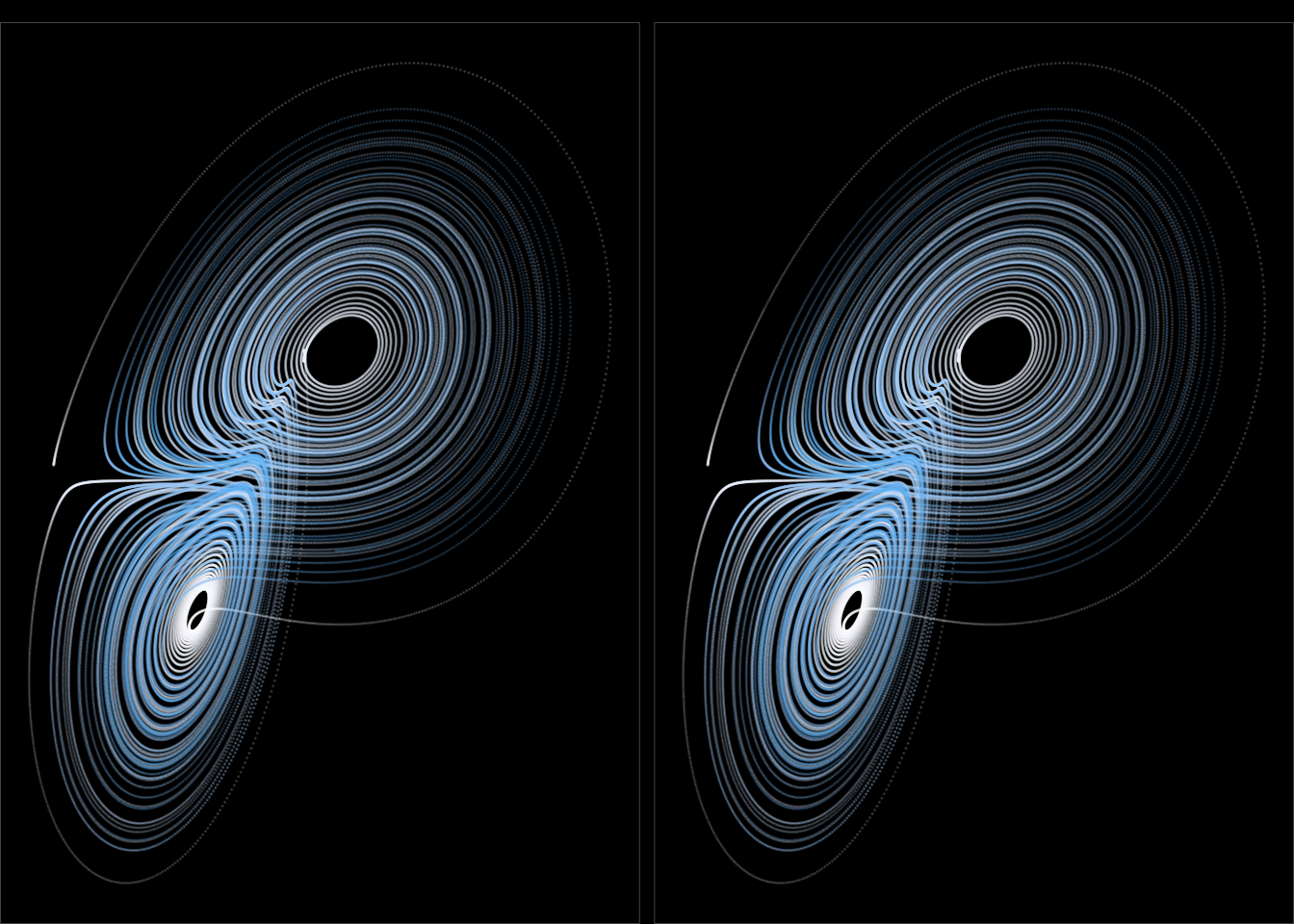
I find it easier to see the image with a black background and lighter shapes. I also draw a thin border around each image, which I use as reference lines when I try to align the two images.
Gallery
That’s all there is to it! I’m still experimenting with how to make viewing easier. When I plot actual data, I’ve found that adding thin lines between some points make for a more convincing illusion.
normalize <- function(v) {
  (v - min(v, na.rm=TRUE)) / (max(v, na.rm=TRUE) - min(v, na.rm=TRUE))
}

data <- datasets::airquality %>%
  mutate(x = normalize(Temp),
         y = normalize(Ozone),
         z = normalize(Solar.R)) %>%
  mutate(depth = z * 0.3,
         shift = 6 * depth / (60 - depth)) %>%
  arrange(runif(length(z)))

bind_rows(data %>%
            mutate(pos = 'left',
                   x = x - shift / 2),
          data %>%
            mutate(pos = 'right',
                   x = x + shift / 2)) %>%
  ggplot(aes(x, y)) +
    geom_path(size = 0.1, color = 'white') +
    geom_point(aes(color = z)) +
    facet_wrap(~ pos, ncol = 2) +
    scale_color_gradient(low = 'white') +
    theme(panel.background = element_rect(color = '#444444', fill = 'black'),
plot.background = element_rect(fill = 'black')) 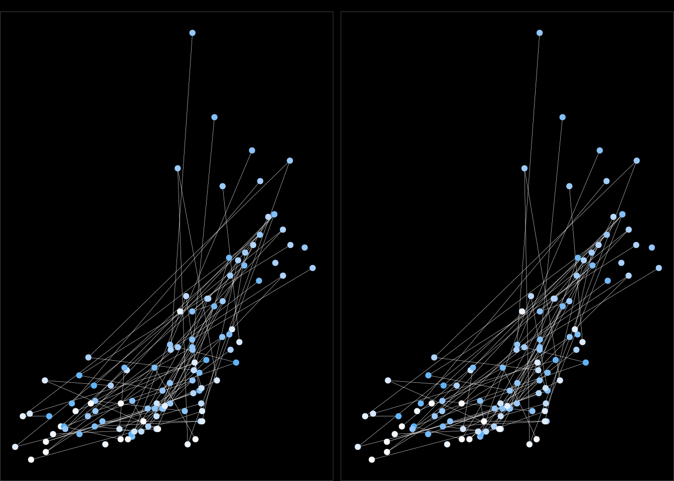
My favorite application is still pretty pictures. Here’s a bunch to practice on.
quadratic_stereo_plot <- function(a, iterations, alpha_trans = identity, color_trans = identity, n_col_trans = function(n, z) n) {
  gridsize <- 500

  data <- iterate(quadratic_3d, a, 0, 0, 0, iterations) %>%
    normalize_xyz() %>%
    group_by(x = round(gridsize*x) / gridsize,
             y = round(gridsize*y) / gridsize,
             z = round(gridsize*z) / gridsize) %>%
    summarize(n = n()) %>%
    ungroup() %>%
    mutate(depth = z * 0.6,
           shift = 6 * depth / (60 - depth))

  bind_rows(data %>%
              mutate(pos = 'left',
                     x = x - shift / 2),
            data %>%
              mutate(pos = 'right',
                     x = x + shift / 2)) %>%
    mutate(n_col = n_col_trans(n, z)) %>%
    ggplot(aes(x, y)) +
      geom_point(size = 0, shape = 20, aes(alpha = alpha_trans(n), color = color_trans(n_col))) +
      scale_alpha(range = c(0.0, 1), limits = c(0, NA)) +
      facet_wrap(~ pos, ncol = 2) +
      theme(panel.background = element_rect(color = '#444444', fill = 'black'),
            plot.background = element_rect(fill = 'black'))
}
a <- c(-0.1, 1.01, -0.43, -0.76, -0.28, -0.09, 0.69, 0.85, -0.16, -0.86, 0.91, 0.04, 1.1, 0.18, -1.12, -0.66, -0.38, 0.81, 0.35, 0.19, 0.12, 0.18, -0.9, 0.45, 0.53, 0.14, 0.12, -1.08, 0.18, -0.91)
quadratic_stereo_plot(a, 300000, alpha_trans = sqrt, color_trans = log) +
scale_color_gradient(low = 'white', high = 'orange')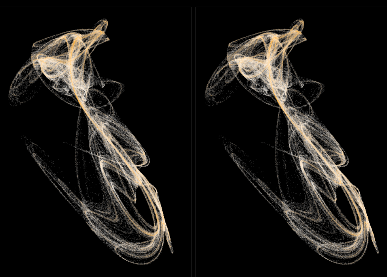
a <- c(-0.35, 0.14, 0.08, -0.78, -1.05, -0.2, -0.12, -0.59, 0.06, 0, -0.62, 0.38, 0.57, 0.31, -0.25, 0.51, 0.93, -0.91, -0.55, 1.01, 0.64, 0.32, -0.72, -0.31, 0.03, 0.3, 0.84, -0.86, 0.49, -0.07)

quadratic_stereo_plot(a, 300000, alpha_trans = sqrt, color_trans = function(z) z^0.3) +
  scale_color_gradient(low = 'white', high = 'green')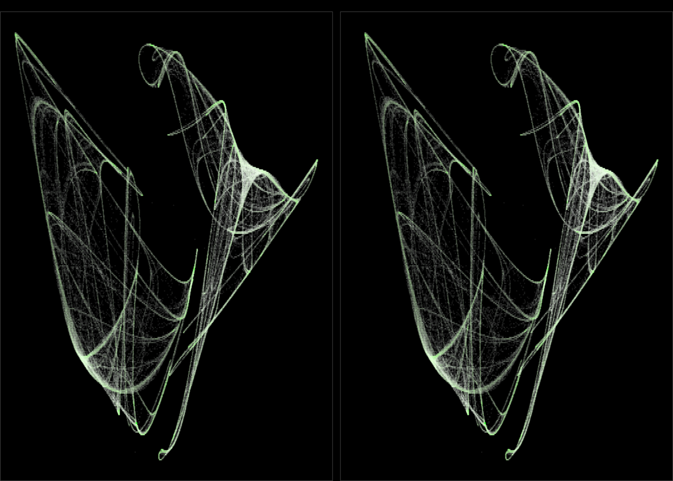
a <- c(-0.48, -0.4, 1.03, 0.62, 0.48, -0.57, 0.26, -0.97, -0.32, 1.05, 0.42, 0.51, -0.51, 0.7, 0.16, -0.55, -0.54, -0.37, 0, 0.65, -0.2, -0.51, -0.29, 0.18, -0.51, 0.37, 0.22, 0.96, -1.03, -0.68)

quadratic_stereo_plot(a, 300000, alpha_trans = function(z) z^0.4, color_trans = sqrt) +
  scale_color_gradientn(colors = rev(lapply(colourlovers::clpalette(131576)$colors, function(c) paste0('#', c))))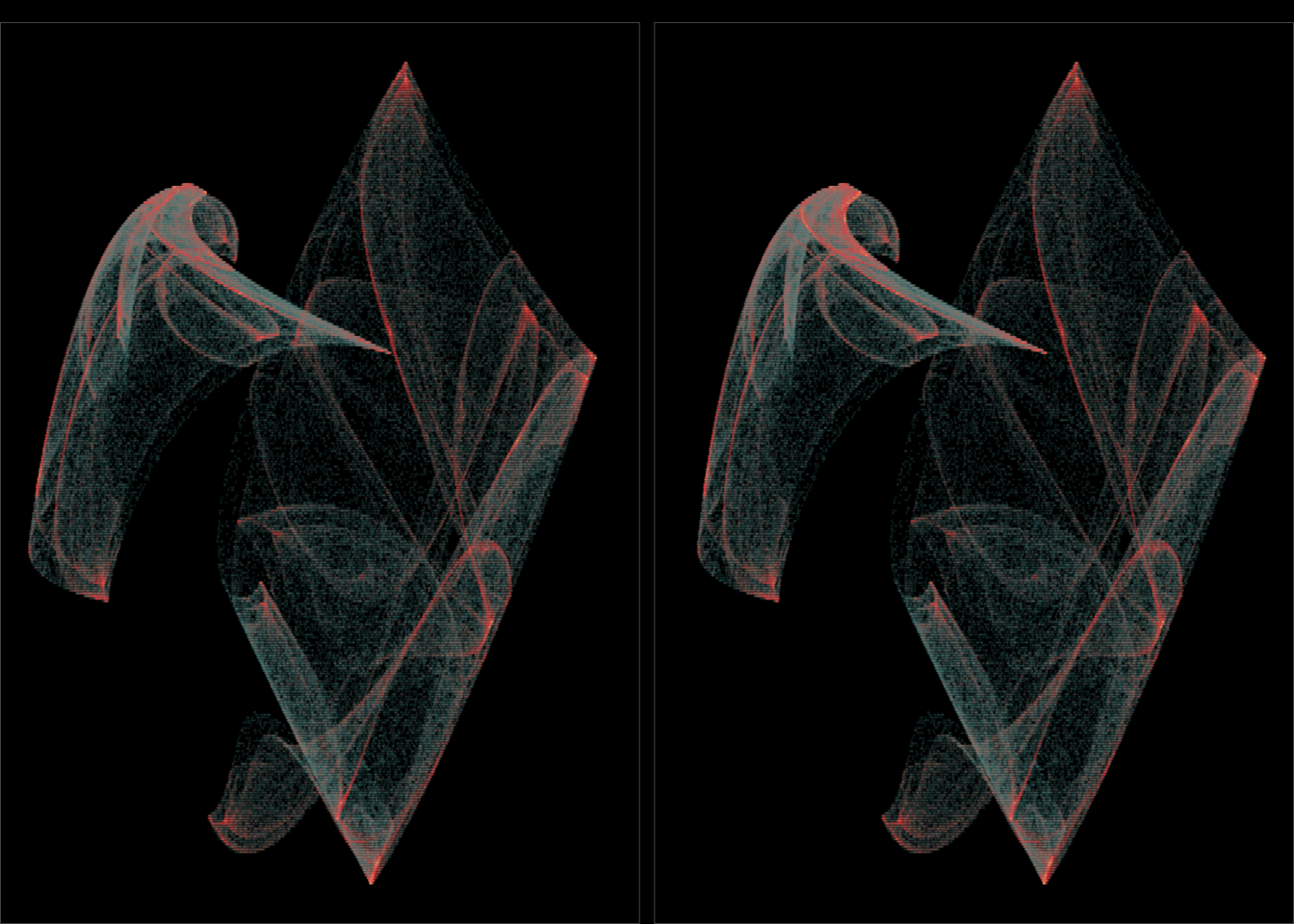
a <- c(-1.08, -0.2, 0.59, 0.03, -0.83, 0.51, -1.01, 0.33, -1.15, -0.89, 0.45, -0.87, -0.36, 0.44, 0.34, -0.28, 0.2, -0.4, 0.49, 0.66, 0.04, 0.13, -0.47, -0.84, -0.32, -0.08, 0.66, 0.54, -0.18, -0.93)

quadratic_stereo_plot(a, 300000, alpha_trans = function(z) z^0.4, color_trans = sqrt) +
  scale_color_gradient(low = 'white', high = 'orange')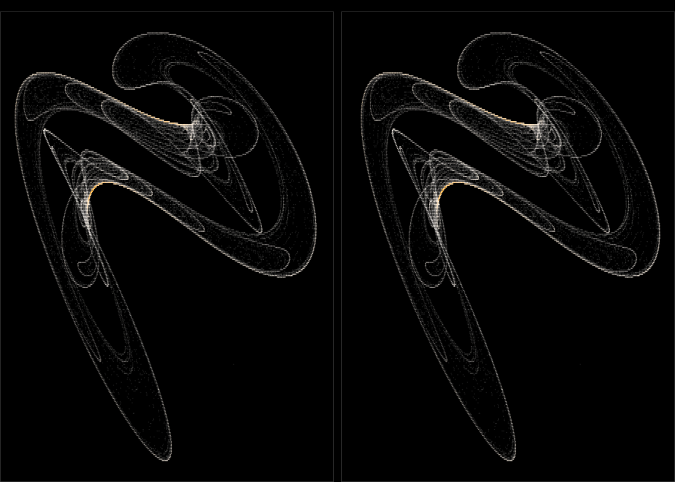
a <- c(0.67, 0.2, -0.97, 0.03, 0.81, -1.05, -0.32, -0.25, 1.09, -1.03, 0.72, 0.87, -0.66, 0.21, 0.25, -1.18, -0.56, -0.22, 0.57, -0.04, -0.19, -0.03, 0.09, 0.54, -0.42, -1.18, 0.37, -0.72, 0.61, 1.01)

quadratic_stereo_plot(a, 300000, alpha_trans = function(z) z^0.9, color_trans = function(z) z^0.7) +
  scale_color_distiller(palette = 'Oranges', direction = -1)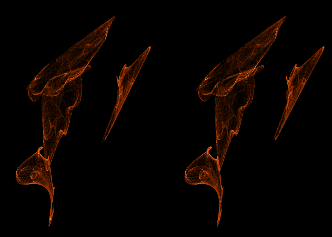
a <- c(0.46, -1.15, 0.38, 0.22, -0.68, -0.11, 0.7, 0.39, 0.49, -1.13, -0.44, -0.83, 1.05, -0.05, 0.13, -0.4, 0, -0.89, 0.73, 0.49, -0.42, 0.02, -0.17, 0.91, -1.11, -0.44, -0.03, -0.94, -0.98, 0.2)

quadratic_stereo_plot(a, 300000, alpha_trans = log, color_trans = sqrt) +
  scale_color_distiller(palette = 'Spectral', direction = 1)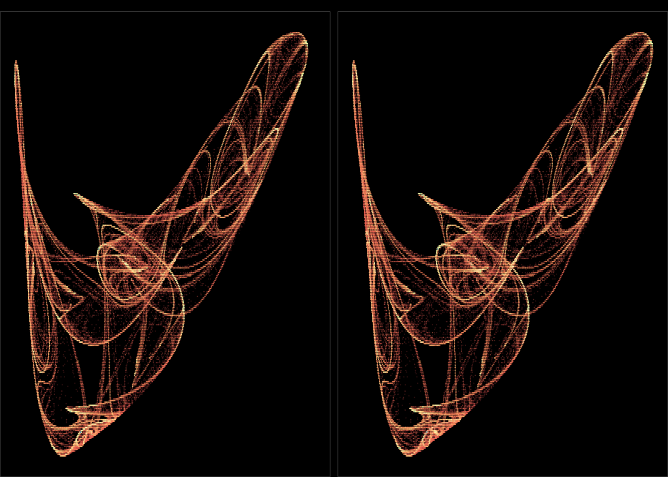
a <- c(0.11, 0.08, 1.04, 1.2, 0.28, 0.24, -1.15, -0.26, -0.96, -0.87, -0.38, 0.05, 0.75, -1.16, -0.03, -1.2, -0.99, -0.42, -0.38, 0.43, 0.01, -0.97, -0.11, 0.92, -0.25, 0.23, 0.53, 0.77, -0.15, 0.79)

quadratic_stereo_plot(a, 300000, alpha_trans = log, color_trans = function(n) -log(n), n_col_trans = function(n, z) ifelse(z < 0.4, n, 5000 * n)) +
  scale_color_gradientn(colors = lapply(colourlovers::clpalette(848743)$colors, function(c) paste0('#', c)))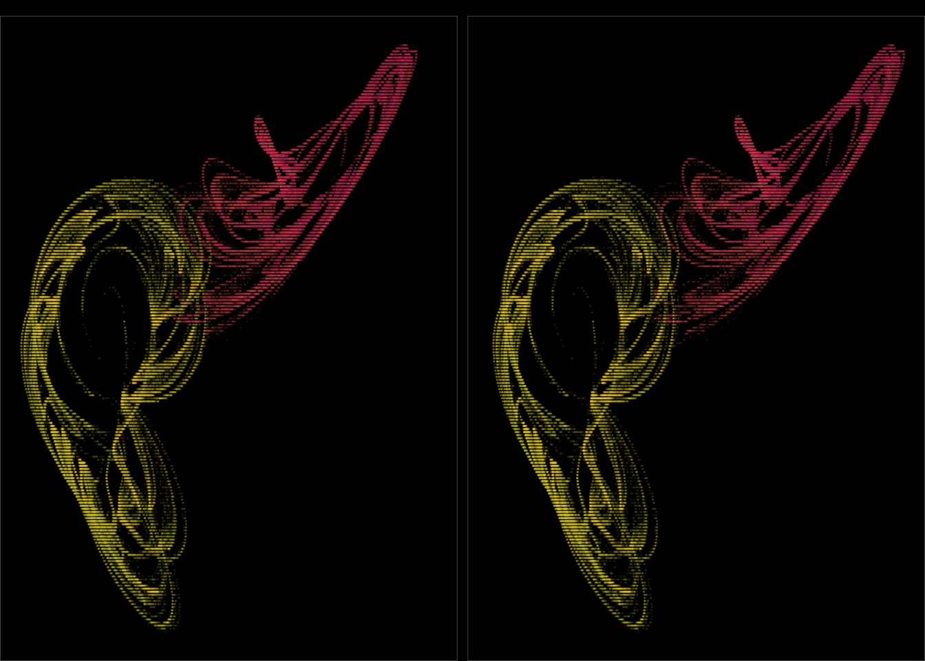
End
If you want to go hunting for 3D images yourself, there is code for 3D hunting that match my description in the 2D post hidden in this documents original .Rmd notebook.
Image credit: Wikipedia↩